A city chart can make a modest numerical change occupy a large visual difference. The numbers need not have been altered. For this original example, imagine a fictional library reporting 100 visits in Period A and 110 in Period B. These are invented counts, not records from a named library. Two proposed bar-chart designs use precisely those totals. Their different baselines explain why looking only at the bars can give the wrong account of what changed.
| Design | Axis range | Visible bar heights above baseline | Actual totals |
|---|---|---|---|
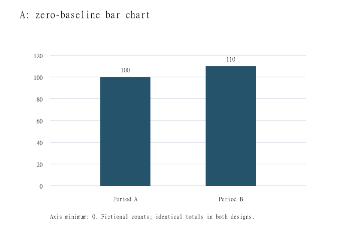
| A: zero baseline | 0 to 120 | 100 and 110 | 100 and 110 |
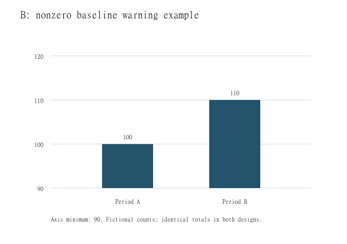
| B: warning example | 90 to 120 | 10 and 20 | 100 and 110 |
Keep the little dataset fixed
Both designs assign the same two periods to the horizontal axis and count visits on the vertical axis. Neither adds a third period, changes the definition of a visit or changes the order of the labels. The numerical difference is ten visits. Relative to the first total, that is an increase of ten divided by one hundred, or ten percent. It is not a doubling of visits.
These are deliberately bare counts. They do not establish how many individual people came, how long the periods lasted or whether an intervention caused the difference. A repeat visitor could contribute more than one visit under an imagined counting system. The exercise isolates the drawing choice rather than filling those missing facts with a city success story.
Design A gives zero a place
In the first proposed chart, the vertical axis runs from zero to 120, with ticks every twenty visits. The bars rise from zero to 100 and 110. With the same plotting height for each design, the second bar is only a little taller than the first. Its length is 1.1 times the first bar, matching the relationship between the totals.
The direct labels remain important: Period A, 100; Period B, 110. Someone reading the chart should not have to estimate exact totals from pixels. A neutral heading can say that fictional visits rose from 100 to 110. That sentence reports the stipulated difference without deciding whether ten additional visits matter to the imagined library.
Design B cuts away the shared first ninety
In the second proposed chart, the vertical axis begins at ninety and ends at 120. The visible bars extend ten and twenty units above that baseline. The second visible segment is therefore twice the height of the first, although 110 is not twice 100. Both numerical labels remain correct; the misleading shortcut is treating the visible lengths as the totals.
The ninety baseline is explicitly labelled, so the design can be inspected rather than mistaken for an unmarked manipulation. It is included here as a warning example, not a recommended presentation. Government Analysis Function guidance advises starting bar charts at zero and explains that a nonzero start exaggerates differences in bar lengths. It suggests a dot plot instead when a close comparison tempts a broken bar axis.
Separate an enlarged difference from an explanation
An editor considering either drawing can ask two different questions: what do the totals say, and what does this visual construction emphasize? The zero-based version preserves the bar-length ratio. The ninety-based version spends most of its visible range on the ten-visit difference. Changing the framing does not add another observation or demonstrate a lasting trend.
For a real report, the period definitions, counting method and source would still need to be supplied. There could also be uncertainty or comparability problems, none of which this invented pair estimates. The useful result here is concrete: read the starting tick, compare the printed totals and calculate the difference before accepting a dramatic visual description.
Sources & further reading
Published sources for the details and examples discussed in this story.